Managing Non-Modellable Risk Factors under FRTB

By Sanjay Sharma, Ph.D. – Chairman, GreenPoint Financial

FRTB allows for RF modelling under IMA only where adequate observable data is available. It prescribes a framework for assessment of the modelability of RFs based on their observability and other factors, and for capital charges for NMRFs. FRTB requires that risk factors (RFs) that cannot be derived and evidenced from prescribed “real or committed prices” at defined frequency are treated as non-modellable (NMRF). Capital charge for trading positions associated with NMRFs is based on a specified methodology that entails conservative stress scenarios for each individual RF aggregated on a summative basis at the bank level. While the concept of NMRFs for computation of capital charge under IMA is logical and necessary, the underlying methodology and implementation will be challenging for both banks and supervisors alike, given vast sets of data sources and trading venues, and heterogeneity of instrument characteristics and trading frequencies.

There are three principal checks for appropriate usage of internal models under FRTB: a qualitative evaluation and approval by supervisors of the rigor and robustness of a banks’ overall framework (this includes internal and external model validation); continual observability of underlying RFs through market prices; and frequent P&L attribution tests that check for the alignment of front office and risk models. In this paper, we focus on the concept, practice, and management of NMRFs.

Criteria for price data

The criteria for a price (the fundamental source of an RF) in FRTB guidelines is for it to be “real” and “continuously” available.

A. Test for “reality” of price data

1. It is a price at which the institution has conducted a transaction;
   OR
2. It is a verifiable price for an actual transaction between other arms-length parties;
   OR
3. The price is obtained from a committed quote; (footnote: this is not defined specifically in FRTB but likely to pass regulatory approval as it is based on the concept defined by Markets in Financial Instruments Directive MIFID).
   OR
4. If the price is obtained from a third-party vendor, where:
   1. the transaction has been processed through the vendor;
   2. the vendor agrees to provide evidence of the transaction to supervisors upon request;
   3. the price meets the three criteria immediately listed above, then it is considered to be real for the purposes of the modellable classification.

B. Test for continual observation of “real” price data for RF extraction

1. A RF must have at least 24 observable “real” prices per year (measured over the period used to calibrate the current expected shortfall model);
   AND
2. Maximum period of one month between two consecutive observations;
   AND
3. The above criteria have to be assessed on a monthly basis.

A “real” price that is observed for a transaction can be included as an observation for all RFs concerned i.e. all RFs that are used to model the risk of the instrument that is transacted. Note that this test must be applied to all RFs, from the highest volume which trade continuously (e.g. USD 10Y) to the lowest volume which trade infrequently. While the former should easily pass the requirement, there will be numerous OTC derivatives that will not qualify easily e.g. swaption volatilities for long expiries and tenors.

Computation methodology for capital charge

FRTB specifies that all trading book positions sensitive or exposed to NMRFs should be capitalized individually based on calibrated stress scenarios at the model/desk level with cross-trade and RTD aggregation to be done at the bank/enterprise level. The capital change is computed based on stress/shock scenarios for each NMRF with appropriate liquidity horizons.

The following describes the methodology for computing and aggregating individual NMRF capital charges.

FRTB divides NMRFs into two groups:

1. K-Type – RFs in internal model-eligible desks that are classified as non-modellable.
2. L-Type – credit spread RFs that have been demonstrated by the bank to be appropriate for zero-correlation assumption when aggregating the NMRF losses resulting from uncorrelated idiosyncratic credit risks (UNICR).

The aggregate regulatory capital measure for L (non-modellable idiosyncratic credit spread RFs that have been demonstrated to be appropriate to aggregate with zero correlation) and K (RFs in model-eligible desks that are non-modellable (SES)) is:

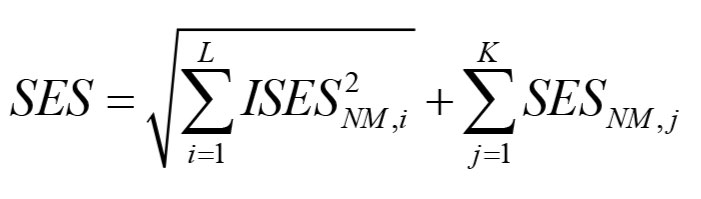
• SES (stressed expected shortfall) is the overall NMRF capital charge
• ISES_NM,i is the stress scenario capital charge for idiosyncratic credit spread non-modellable risk i from the L RFs aggregated with zero correlation
• SES_NM,j is the stress scenario capital charge for non-modellable risk j.

Stress shocks and scenarios have to be calibrated to be at least as prudent as the ES calibration used for modellable RFs, i.e. loss calibrated to 97.5% confidence threshold over a period of extreme stress for the underlying RFs. For each NMRF the liquidity horizon of the stress scenario has to be greater than the longest interval between two consecutive price observations of the prior year, and the liquidity horizon assigned to the prescribed RFs.

Our interpretation of this requirement is that if adequate plausible historical price data is available to calibrate appropriate and acceptable shocks for an individual NMRF, an “ES equivalent” calculation should be acceptable as an RF-specific stress scenario. As data availability becomes sparse, the assumptions for shocks should be made increasingly conservative with longer liquidity horizons. This range can be specified with supervisory approval at 97.5% confidence and ES with holding periods scaling up based on data gaps and liquidity horizons as prescribed under IMA.

If the SES is positive, it will be capped at zero. For large RF shocks, pricing models may produce odd or unexpected results as arbitrage conditions that underlie the specific model change. In this case SES can be computed via a backup approach based on sensitivity.

The internal model capital charge C_A for all desks with internal model approval is calculated based on the scaled expected shortfall and the aggregated NMRF charges using the following formula:

C_A=max (IMCC_t-1+SES_t-1;m_c×IMCC_avg+SES_avg)

Where:

• IMCC_t is the internal model capital charge calculated with the scaled expected shortfall model at time t
• SES_t is the aggregated NMRF charge as described above, and m_c is a multiplier that is set individually for each bank by the regulators with a floor of 1.5

NMRF capital charge principal contributing factors

Initial estimates point to NMRF capital charge being significantly higher than for ES-based IMA capital charge for modellable RFs. This stems from a combination of three underlying FRTB methodology prescriptions:

1. Conservative stress scenarios Under FRTB, capital charge for NMRFs has to be computed based on conservative stress scenarios proposed by banks and approved by supervisors.
2. Longer liquidity horizons The liquidity period for NMRF capital charge is assumed to be longer of the proposed risk class-specific charge prescribed under IMA, or the time period between the two “real price” quotes that are most further apart over the prior year.
3. Limited correlation, diversification and hedging benefit at the RTD level. FRTB prescribes that correlation or diversification benefits across NMRFs are to be netted and adjusted for at the bank level. The genesis of this is that because NMRFs arise from endemic or episodic absence of verifiable real prices, and making correlations between NMRFs and across modellable RFs are difficult to estimate reliably.

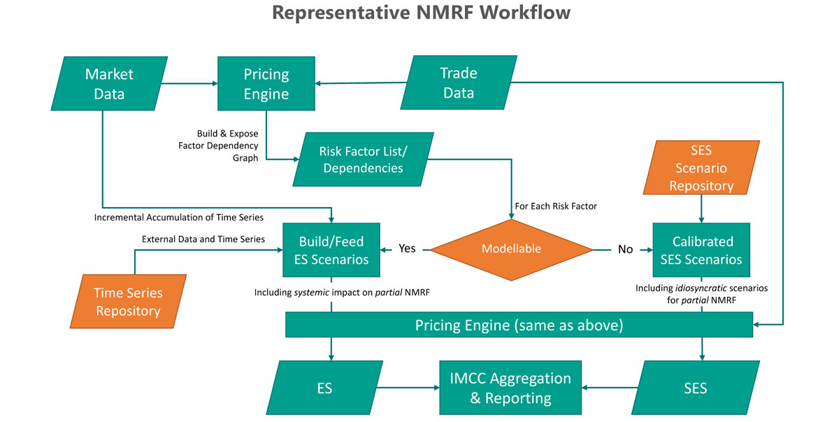
NMRF workflow

For desks that are deemed eligible for internal model approval the underlying RFs for each model will be categorized vis-à-vis their observability in the RF analysis process. RFs that can be objectively verified using “real prices” are hence classified as modellable and capital charge can be computed through the ES approach. All other RFs are categorized as non-modellable and are to be capitalised using the NMRF charge, based on individual stress scenarios and a conservative aggregation framework.

Addressing the NMRF compliance obligation for banks will have several components requiring both sequential and simultaneous workflows.

The panel below illustrates a high-level process for management of NMRFs.

We describe a three-step RF identification methodology for establishing an FRTB compliant RF framework.

Implementing a systematic identification process

A bank’s NMRF identification process should be focused on objectively validating RF values based on real transactions. To that end, the identification process can be divided into three steps:

A. Identify relevant RFs

All relevant RFs of a bank’s trading book portfolio should to be identified in a structured and comprehensive manner on a regular basis for all trading desks eligible for IMA based on a common RF definition.

RFs that are omitted from internal models (i.e. both for the Expected Shortfall and NMRF calculations) should be flagged. The omission should be justified and documented as prescribed by jurisdictional supervisors, e.g. by providing the appropriate P&L attribution test statistics.

B. Create instrument to RF Mapping

1. Modelability assessment of individual RFs is based on “real prices” of representative transactions. Towards that end, a mapping between RFs and representative products should be defined. This mapping should link RFs to instruments with demonstrable materiality and tractable relationship between an RF and the price of the respective instrument. Generally, several instruments may be available to evidence the same RF.
2. Identification and regrouping of RFs

The list created in Step 1 should be redrawn to identify common RFs and their sources based on commonality, materiality, frequency and robustness.

This analysis has to be performed across all internal and external data sources. The most optimal combinations of RF sources and price data can be identified, listed and prioritized for each model.

3. Calibration of models with new RF sourceIn situations where a unified model framework and RF mapping involves changes, calibration should be performed to ensure compatibility and avoid surprises.

C. Selection and inclusion of RFs

Listing and grouping of existing models with FRTB prescribed risk buckets. Since 2008, banks’ model organization and validation documentation for risk models have undergone substantial transformation as required by supervisory bodies. However, given the flexibility provided to banks under Basel 2.5 IMA, current model frameworks are siloed by asset class, trading desks and business units. Siloed frameworks are not conducive for RF identification and NMRF minimization under FRTB. It is strongly advisable that were it does not exist, banks conduct a comprehensive listing and categorization of individual risk and pricing models along with RFs and their sources.

D. Observability check

Any “real price” that is observed for a transaction should be counted as an observation for all the RFs concerned i.e., all RFs which are used to model the risk of the instrument that is bought, sold or generated through the transaction as part of the overall portfolio.

To check observability, “real price and committed quote” data can be sourced from internal transactions or third parties. In the latter case, the data will most likely be procured from a vendor, who can process the transactions and record the necessary observability evidence and audit trail that can be provided to supervisors by the banks. The “real price” data is then projected back onto the RFs to assess their modelability based on the mapping rules created in the previous step.

Qualified price observations are mapped to the RFs and two data fields are recorded: the count of observations within the last year; and the longest gap between two consecutive observations. Mapping has to be done such that instruments and transactions have to be linked to specific RFs across materiality and historical consistency availability of prices. It will be possible to link several RFs to a single instrument across risk class buckets and asset class. This classification can be guided by the SA risk class bucket classification and IMA liquidity buckets.

The following steps can then be followed:

1. If the data is near fail thresholds examine alternate RF sources and substitute with impacted capital.
2. If other RF sources are also close to the disqualifications range qualifying prepare to apply proxy and basis. This will increase the capital charge because of the NMRF charge associated with the non-modellable basis.
3. Although FRTB does not allow for transfer of trades across desks future trades should be booked under SA desks.
4. If IMA capital charge is high with NMRFs, create a process for adopting SA.

Considerations

To summarize, the following three considerations for utilizing the flexibility afforded under FRTB for RF selection should be integral to the workflow:

1. Systematic approach

   The mapping between RF sources and instruments should be systematic and thorough. If not well planned and executed the flexibility to select RFs from multiple sources can result in a disorganized model environment with ad hoc choices lead to inconsistency that may be hard to document and justify to supervisors.

2. Materiality

   Due consideration given to materiality of RFs factors in the valuation and risk models. Defining the materiality of RF can be a straightforward sensitivity assessment of simulated movement in prices vs. redefined RFs across alternate instruments.

3. Reliable frequency of the real prices of source instruments

   The choice of instruments as RF sources should incorporate their historical trading volume and frequency of the availability. At a minimum, the choice of RF sources is a balancing and organizing act.

Additional points for RF selection

Market data that is used to illustrate RF modelability may not be suitable for computing ES. Once an RF is proven to be modellable, banks are allowed to use all available data sources to calibrate an internal model.

Categorization of RFs for NMRF are allowed to be distinct from other representations. For instance, in a standard volatility model, e.g. SABR, the parameters of the volatility model are considered as RFs. The underlying parameters of these models are calibrated from swaption prices with combinations of expiry, tenor and strike/moneyness.

1. Under FRTB, if the underlying parameters are demonstrably derived from modellable RFs with “real price” and specified observation frequency, the calibrated parameters are clearly modellable as well. For instance, for interest rate derivatives, the underlying RFs can be extracted from interest rate volatility surfaces for each currency demonstrate the availability of price data for applicable and modellable transactions then the SABR models can be used.

The following sections provide guidelines on computation of capital charge, selection and management of RFs and calibration of shocks that incorporate appropriate liquidity horizons.

Strategies for NMRF management and optimization

The conservative aggregation structure prescribed by FRTB scales linearly with the number of NMRFs and can result in economically unrealistic NMRF capital charges. As no diversification benefits are granted across NMRFs, banks would be less motivated to hedge and diversify their portfolios. If an NMRF is hedged with a modellable RF, the overall capital consumption can potentially become very punitive. Positions with NMRFs will have to be capitalized on a standalone basis, separate from associated hedges leading to an additional capital charge as part of the Expected Shortfall calculation. This implies that FRTB will lead to economically sensible risk management and hedging strategies being discouraged due to a potentially punitive capital treatment wherein a hedged portfolio has a higher capital consumption than a non-hedged portfolio.

To mitigate these undesired effects, several techniques can be employed that are provided below. We describe and illustrate some straightforward methodologies below.

A. RF decomposition

FRTB allows for the decomposition of NMRFs into modellable benchmarks and “residual basis” that would be capitalized as non-modellable. This is logical because RFs that are observable generally have an underlying basis that is modellable. The simplest example is the case of a corporate bond wherein idiosyncratic credit risk in the mind of a trader/investor is generally relative to that of an index or other liquid bonds. In these cases, the additional risk premium that may be truly non-modellable is an add-on to the other components that include credit risk of similar issuers and prevailing interest rates, i.e. credit risk spread for small and illiquid issuers can be decomposed into a liquid credit spread index that is modellable to which a nonmodellable basis or spread is added. In a similar fashion, long tenor points for interest rate curves that may not be frequently traded and observed and do not pass the observable price criteria can be decomposed into shorter-tenor observable points and cross-tenor basis spread.

Banks and RTDs should consider the following general guidelines for decomposing NMRFs. Several factors will determine if the decomposition of a RF is more capital efficient than modelling the non-modellable RF as an outright NMRF:

• Proportional variation of the NMRF that can be explained by the modellable RF proxy.
• Relative size of the trading book/position vis-à-vis risk offsets.
• Chosen proxies should have a demonstrable causal relationship with the modellable proxy that can be observed and recorded on a regular basis.
• The RTD should be prepared to reduce the overall NMRF positon in case there is an episodic divergence with the modellable proxy and unexpected increase in the NMRF capital charge.
• The relative sizes of NMRF and proxy positons that are balanced and managed as a “pair trades.” This function can be extended to an NMRF portfolio but only with sophisticated risk management and FRTB systems.
• Proxies should be chosen carefully with due consideration to the balance between their liquidity and proximity to the NMRF. In general, a well-chosen liquid single-name CDS as a proxy will have a smaller basis compared to a CDS index, and thus lower volatility and lower NMRF capital charge.
• A proxy itself may have high volatility resulting in a net increase in NMRF capital charge. This can be true of an index as well.
• The proxy may itself become non-observable to the capital charge.
• Particular attention should be paid to instrument specific idiosyncratic risks that may not be proxy-able. Consider the case of credit risk of a corporate bond is represented across the following RFs:
  1. Issuer-specific default probability
  2. Recovery rate
  3. Issue-specific idiosyncratic risk

The default probability and the recovery rate can both be observed from bonds of the same issuer with identical seniority and maturity. However, the issue-specific idiosyncratic risk of the the specific bond can only be observed from market prices of bonds that have the same default provisions, other terms, and covenants, etc

B. Calibration of stress scenarios for computation of SES

RFs classified as non-modellable must be capitalized at the bank level, based on stress scenario for each NMRF. We suggest a methodology for calibrating shocks according to FRTB guidelines and applicable liquidity horizons. These shocks drive the computation of capital charge individually for each non-modellable RF.

FRTB requires that stress scenarios used for computing capital should to be calibrated to be “at least as prudent as the expected shortfall calibration used for modeled risks (i.e. a loss calibrated to a 97.5% confidence threshold over a period of extreme stress for the RF value)”.

Our interpretation of this requirement is that if sufficient data is available to calibrate an appropriate shock for an individual NMRF, an ES-equivalent calculation would be sufficient as an RF stress scenario. However, as data availability becomes scarce, more conservative shock approaches for stress must be used. Where a modellable RF is not available during the historical period used for stressed calibration (e.g. 2007-08), proxy data can be used, provided the general approach for replicating missing data is justified and documented as part of the independent review of the internal models, as well as approved by the bank’s supervisory body. Although the FRTB guidelines have not stated this explicitly, it should be noted that this does not apply to ongoing observation and validation of data availability.

A rational and practical approach is to reprice all instruments for which the models are impacted by the NMRF classification as an impact with calibrated stress scenarios at 97.5% confidence level. The stressed expected shortfall is computed by shocking the RF twice with same parameter interval up and down. The higher loss of the two scenarios is selected at the bank level.

We propose a three-step for creation and calibration of SES.

1. If an applicable historical time series is available, the NMRF shock should be calculated over a period of stress for the specific RF1 as an expected shortfall at 97.5% confidence level.
2. If the historical market data is unavailable and/or is of poor quality, the maximum loss observed over the liquidity horizon should be used as stress scenario.
3. For cases where the historical market data is incomplete and unreliable such that the justification for its usage is questionable, the bank should calibrate the stress scenario based on expert judgement based on historical and or hypothetical assumption sets.

All stress scenarios have to be approved by banks’ supervisors. If they do not deem a stress scenario to be sufficiently conservative, they can ask for an NMRF capital charge equivalent to a maximum loss of the principal amount at risk

C. Mechanism for “break-glass” SA fallback

SA is designed to be the IMA fallback under FRTB. In situations where the alternatives for managing NMRFs are cumbersome or not robust, SA can be a feasible alternative. The capital change will be higher than IMA, but not if the NMRF component is large.

The decision to select SA for an RTD can be based on the following comparison criteria:

1. The relative impact of correlation assumptions under IMA/NMRF (which can be zero for demonstrably non-correlated credit risks)
2. The comparison between SES scenarios under NMRF capital change computation vis-à-vis prescribed risk weights in SA

It should be noted that for idiosyncratic credit risk the comparison may not be tractable because of the size of proxies for NMRF computation. This is because the concept of an inherently a non-zero correlation. Thus, by using a shared proxy across idiosyncratic credit risks is unspecified (correlation assumption a zero). The impact of proxy-related correlation would be diluted at the bank-level e.g. computation can also be hedged perfectly with liquid credit investments. A quantitative comparison algorithm can be designed that incorporates SA risk weights, correlations, regression R squared the impact of proxies and residual variances.

Summary

Management of NMRFs and P&L Attribution Tests are where the FRTB rubber meets the capital road. It is very likely that BCBS will make this road smoother by providing clarity and more rational criteria for IMA implementation and regulation. However, it is highly unlikely that these tests will be withdrawn from FRTB. Banks and trading desks will do well to be armed with flexible technology systems and models framework to face the bumps on the road and ensuring a smooth ride towards capital optimization.